PUBG Placement Prediction
CS 7641 Team 6: Jas Pyneni, Hemanth Chittanuru, Kavin Krishnan, Vishal Vijaykumar, Rafael Hanashiro

1. Overview
PUBG is a battle-royale video game where 100 players battle on a game map by rummaging for weapons and tools and fighting until there is only one surviving player or team. Initially a Kaggle competition, the purpose of this project is to predict the final placement of a given player based off of game stats. This is an interesting project for our group because it is a game we all love to play. We hope that by applying the skills we learned this semester in CS 7641, we can learn the best way to maximize our chances of winning our future matches. So far, winning has been determined by starting randomly and employing different in-game tactics, but by doing this project, we can learn with ML how to win.
We feel that we can solve our problem by verifying that our data is valuable and are confident in the techniques we learned this semester to find that value. Instead of individually getting better at various in-game tactics, we hope to build a prediction engine that can tell us how likely a given tactic is to win so we can test out our ideas and focus on winning.
We aim to do this through the following steps:
- Explore the data
- Pre-process and engineer the features
- Model the data and build a prediction engine
2. Data Exploration
Dataset: PUBG Match Placement Data
Collected from Kaggle
4446966 starting stats, 28 features, 1 target
Features:
- Id - unique identifier of player
- groupId - ID to identify a group within a match.
- matchId - ID to identify match
- assists - Number of enemy players this player damaged that were killed by teammates.
- boosts - Number of boost items used.
- damageDealt - Total damage dealt - self inflicted damage
- DBNOs - Number of enemy players knocked.
- headshotKills - Number of enemy players killed with headshots
- heals - Number of healing items used.
- killPlace - Ranking in match of number of enemy players killed.
- killPointsElo - Kills-based external ranking of player. (
- kills - Number of enemy players killed.
- killStreaks - Max number of enemy players killed in a short amount of time.
- longestKill - Longest distance between player and player killed at time of death.
- matchDuration - Duration of match in seconds.
- matchType - String identifying the game mode that the data comes from.
- maxPlace - Worst placement we have data for in the match.
- numGroups - Number of groups we have data for in the match.
- rankPointsElo - Elo-like ranking of player.
- revives - Number of times this player revived teammates.
- rideDistance - Total distance traveled in vehicles measured in meters.
- roadKills - Number of kills while in a vehicle.
- swimDistance - Total distance traveled by swimming measured in meters.
- teamKills - Number of times this player killed a teammate.
- vehicleDestroys - Number of vehicles destroyed.
- walkDistance - Total distance traveled on foot measured in meters.
- weaponsAcquired - Number of weapons picked up.
- winPoints - Win-based external ranking of player.
Target:
- winPlacePerc - The target of prediction. This is a percentile winning placement, where 1 corresponds to 1st place, and 0 corresponds to last place in the match.
Feature Characteristics:
- int IDs to identify players, groups and matches
- Discrete data about stats (assists, boosts, headshotKills)
- External rankings (based off of some post-match math): ELO scores
- Certain features listed as inconsistent (rankPointsElo)
Visualization
Feature Analysis
A visualization to show how each individual feature is correlated with the other features
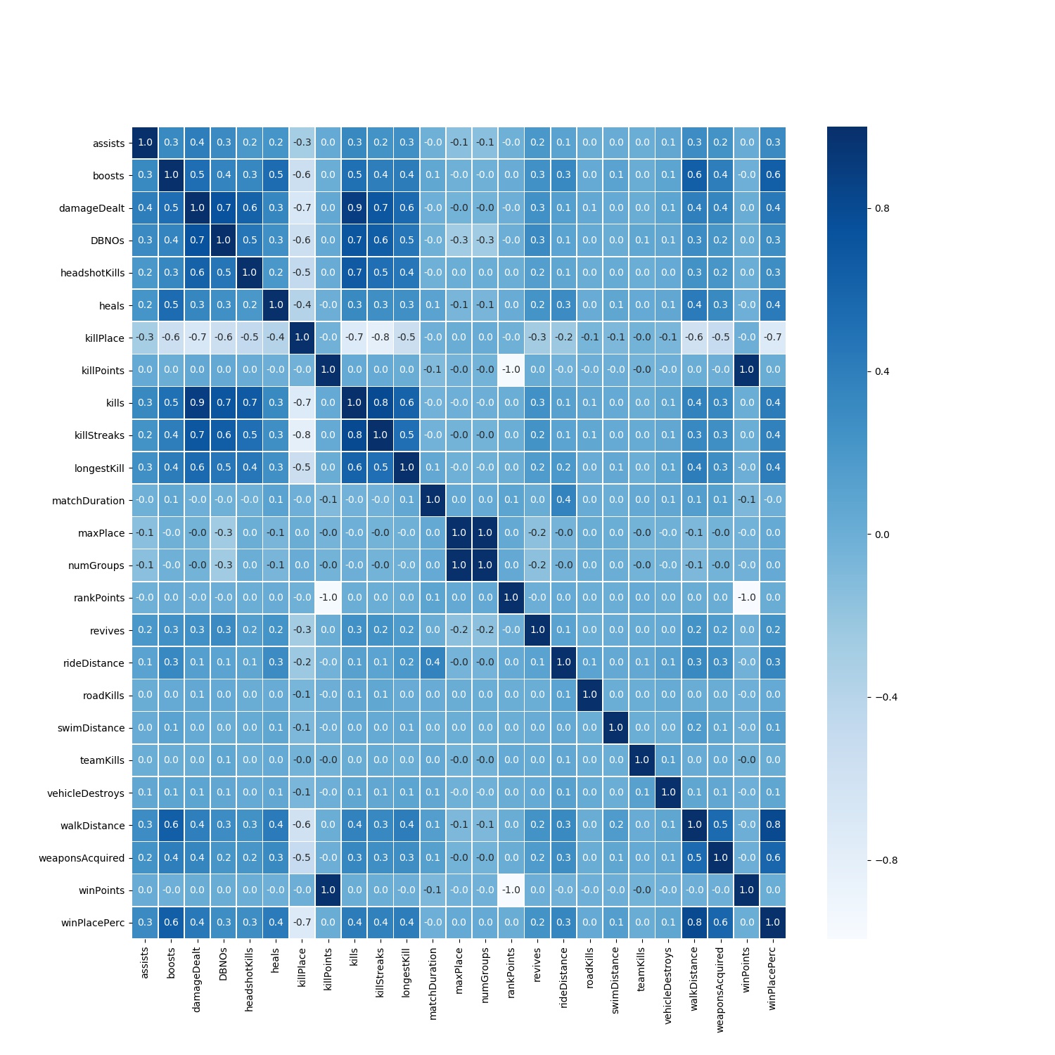
The last column in the above matrix is the most important as it shows the correlation of each feature with our target variable winPlacePerc.
From the heat map we can see that there is a high positive correlation between walkDistance and winPlacePerc. This is interesting and so let’s explore the relationship of all types of traveling totalDistance = (walkDistance, rideDistance and swimDistance) and winPlacePerc.
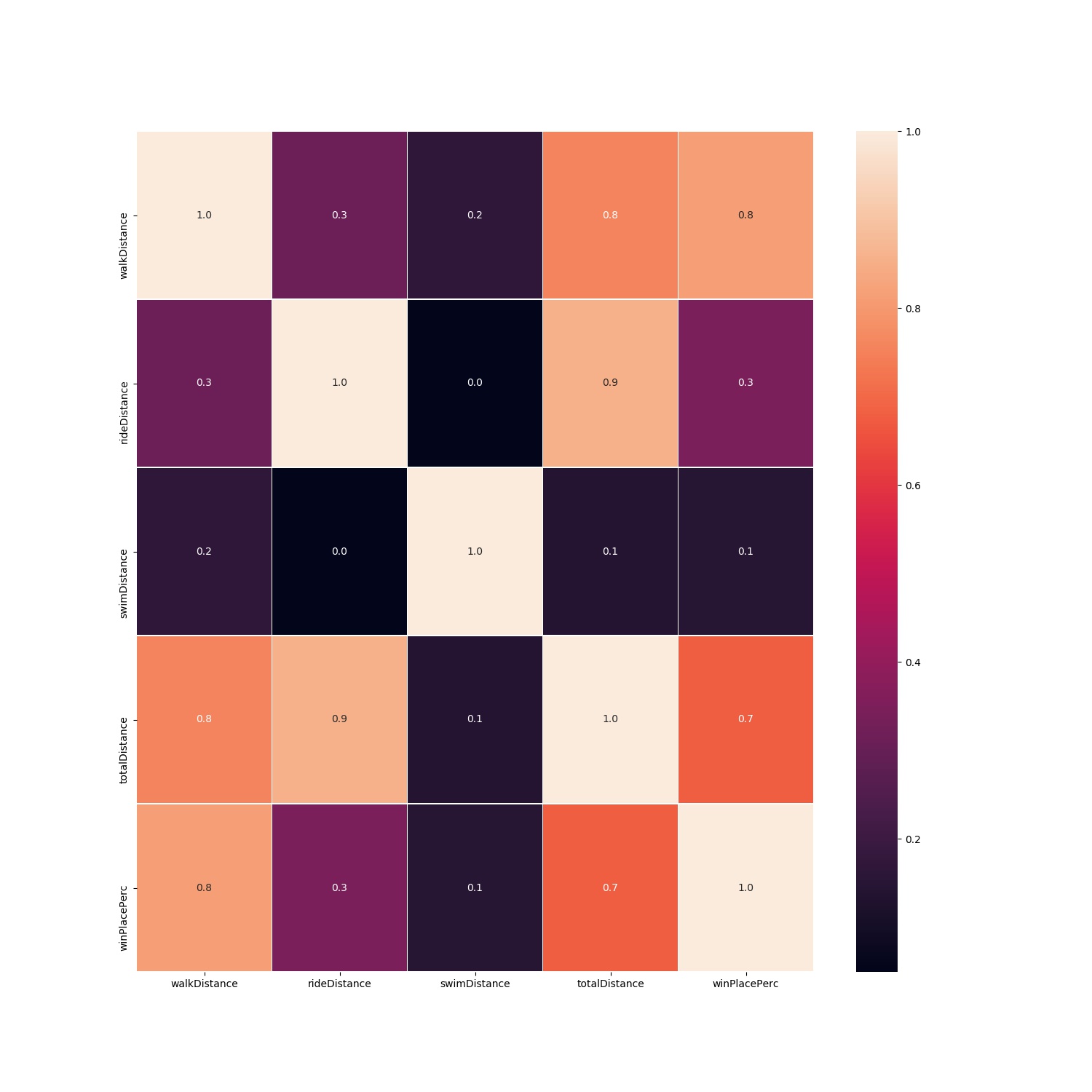
We can see that there is high positive correlation between totalTravelDistance and winPlacePerc as we saw for walkDistance and winPlacePerc.
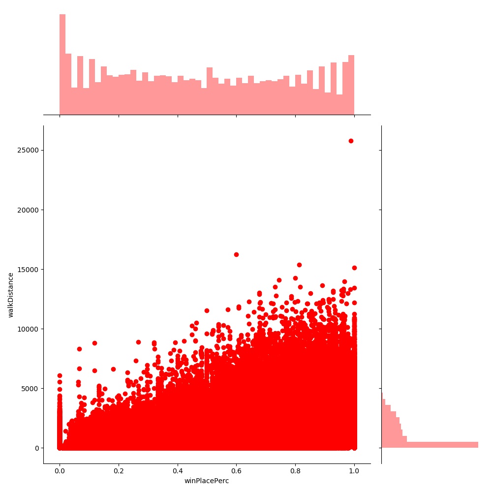
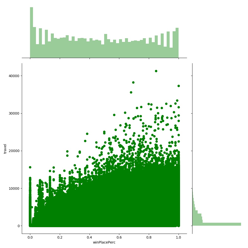
Let’s visualize the positve relation between walkDistance and winPlacePerc as well as totalTravelDistance and winPlacePerc.
walkDistance vs winPlacePerc
totalTravelDistance vs winPlacePerc
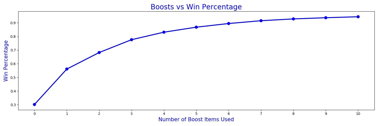
The heatmap also shows a strong correlation between boosts and winPlacePerc. A graph of the central tendency of the two should help us get a better visual understanding of this relationship.
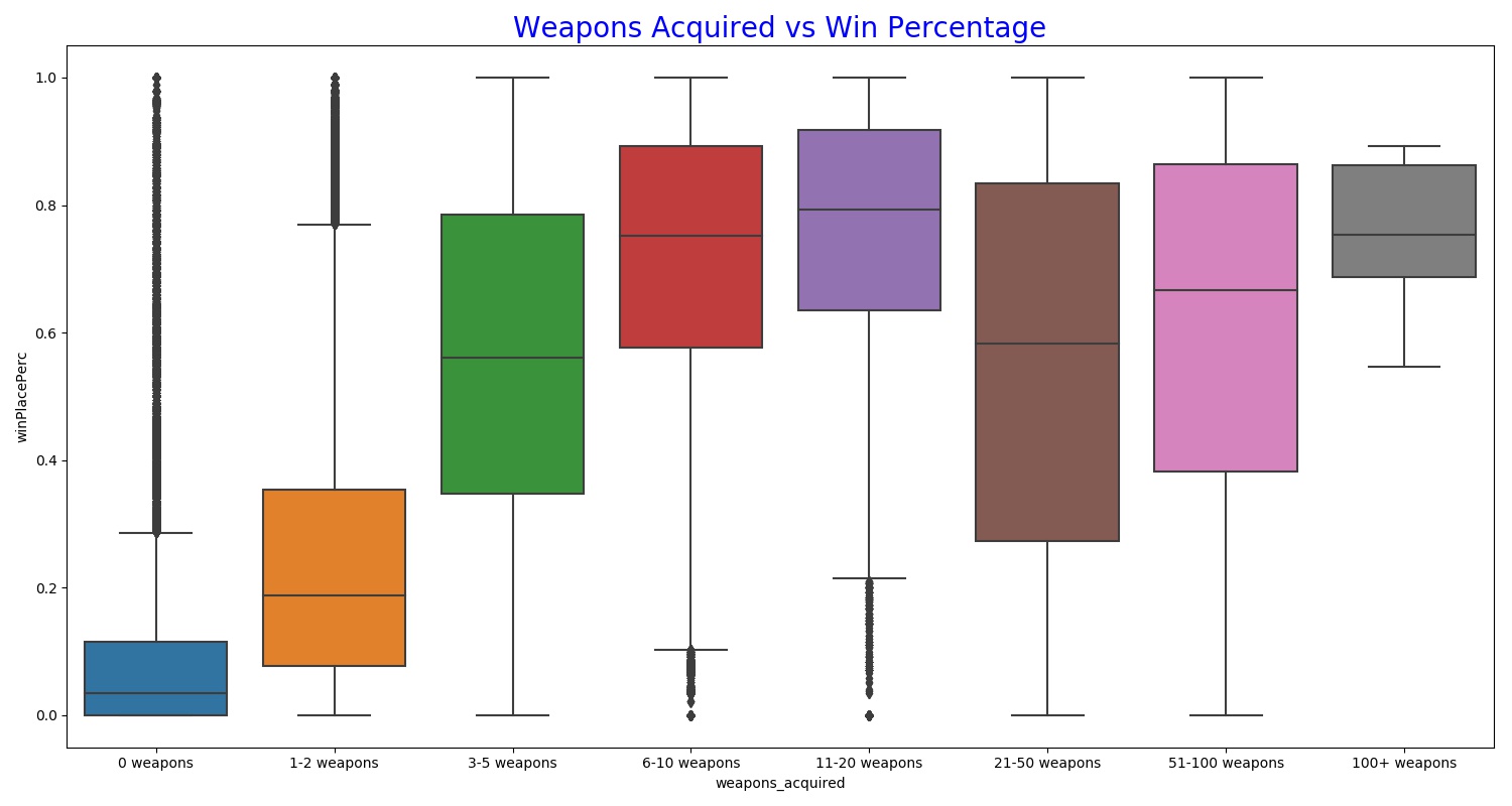
Similarly, there is a relatively high correlation with weaponsAcquired and winPlacePerc.
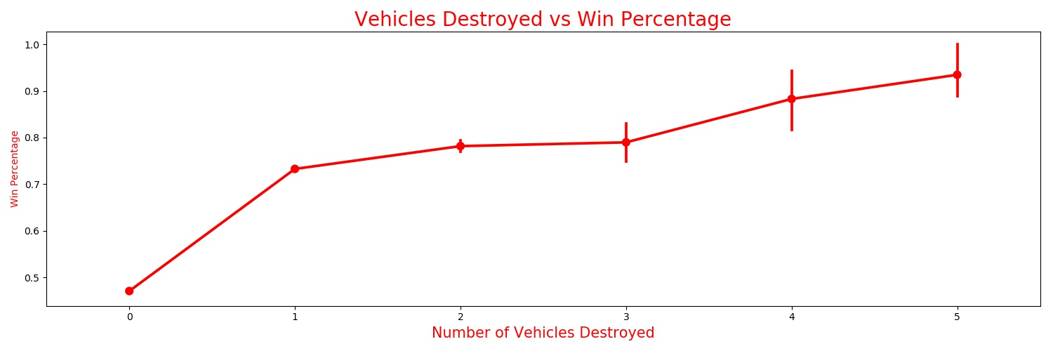
Based off my experience with the game, I know that people that can destroy vehicles tend to be better players.
3. Pre-processing
Based off the above visualizations, we can see that certain features definitely give us a lot of information while others provide no input in terms of our target variable. This allows us to have a basis for using the data and also shows that the data we have is indeed valuable data. This means the next step is deriving the actual value from that data.
As such, we will preprocess the data like this:
- remove presumed irrelevant features: Id, groupId
- One-hot encode match type: solo (one player), duo (1-2 players), or squad (team)
- Drop all rows with NaNs
- Split into train and test such that no instances of same match are in both test and train.
We can choose to manually take out those features that do not seem to be providing any information but we can use dimensionality reduction algorithms to do that for us.
Dimensionality Reduction
We considered two dimensionality reduction methods to reduce the size of our feature space to avoid the Curse of Dimensionality. After one hot encoding our match type during preprocessing, we had 40 features.
Principal Component Analysis
The first dimensionality reduction method we used is PCA. PCA aims to convert a large set of features to a smaller set of uncorrelated features. The below graph plots the proportion of variance to the number of principal components.
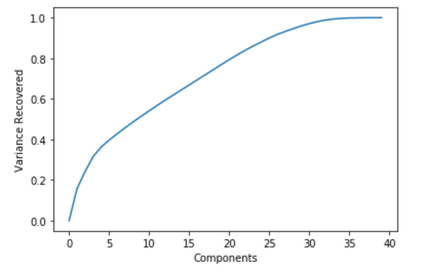
As we can see from the above graph, we were able to recover 99% of the variance by using ~34 principal components.
Random Projection
The other dimensionality reduction method we’re using is random projection, specifically, Gaussian. In random projection, we convert the high-dimensional feature space to a lower-dimensional feature space such that the distances between the data points is conserved. In Gaussian random projection, the matrix used is generated using a Gaussian distribution. To pick the number of components used in this Gaussian Random Projection, we split the training data set into a training and validation set, and trained our model on the feature spaces modified by the random projection, using 2 to 40 components. After this, we tested the model’s performance on the validation set, and plotted the RMSE and MAE.
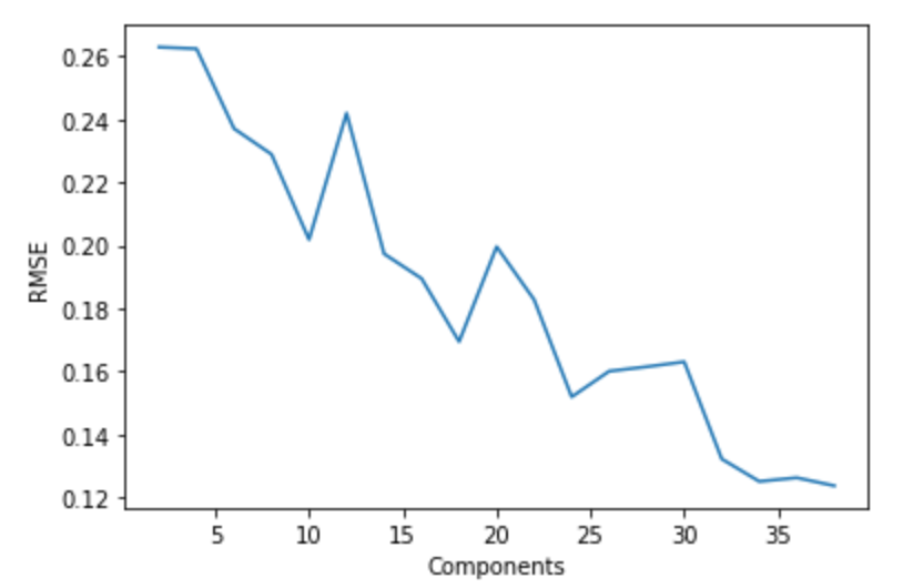
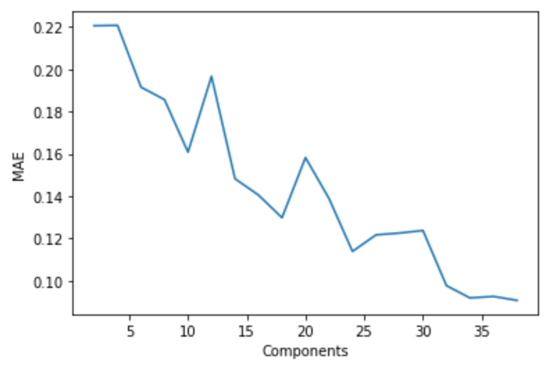
Looking at these graphs and the error values, we see that the error evens out at 34 components.
4. Modeling, Experimenting & Results
a. Gradient Boosting
We used gradient boosting as one of our supervised learning models. Like other boosting methods, gradient boosting combines weak learners to form a stronger and more accurate model. Recently, they have become very popular among Kaggle contestants due to its performance. Here, we used the XGBoost implementation, which follows the principles of gradient boosting but introduces regularization to reduce overfitting and improve performance.
Model Performance
In order to get a better notion of the quality of our model and the effectiveness of our feature engineering, we tested the model on several distinct variations of the dataset.
Before Data Pre-processing
Prior to any dimensionality reduction, we trained our model on the raw data. Due to the nature of XGBoost, it does not handle categorical features, so we removed the features Id, groupId, matchId and matchType. In order to not include any match in both the test and train sets, we performed the test/train split based on matchId. In particular, all data points belonging to a specific matchId would be entirely in either the test or train datasets, where the train split contained approximately 90% of the data.
The default decision tree weak learner and squared loss were used to train the model, and results were the following:
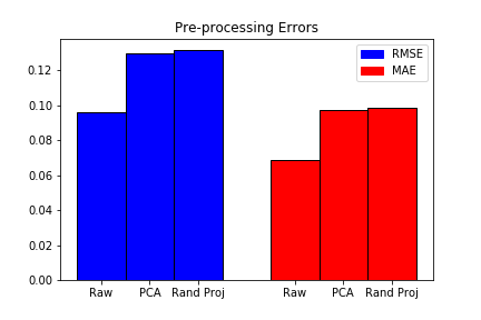
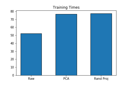
- Time elapsed for training: 52.32 s
- RMSE: 0.09612
- MAE: 0.06894
The Mean Absolute Error (MAE) was the metric used in the Kaggle competition to evaluate contestants.
After PCA
We analyzed the model after performing dimensionality reduction through PCA and obtained the following results:
- Time elapsed for training: 76.54 s
- RMSE: 0.12955
- MAE: 0.09740
After Random Projection
We also analyzed model performance after performing the random projection algorithm, yielding:
- Time elapsed for training: 77.40 s
- RMSE: 0.13181
- MAE: 0.09844
The error and training time for each pre-processing can be seen in the graphs below
Hyperparameter Tuning
The XGBoost algorithm contains several hyperparameters which change the behavior of the model. We tuned 2 of the most important ones, comparing the errors yielded in each case. We used the raw dataset (without any dimensionality reduction or extensive pre-processing) to train the models, since it yielded the best results.
Weak Learners
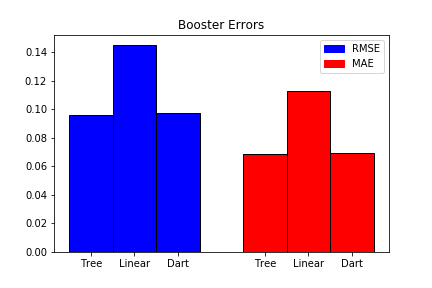
Boosting methods work by combining various weak learners to form a more powerful model. The XGBoost implementation used has access to 3 different types of weak learners: linear, decision tree and dart.
Tree Booster
The tree booster uses decision trees as weak learners. It is the most common approach with the XGBoost algorithm. The model performance was given earlier, as we used it to analyze the different feature engineering techniques.
Linear Booster
The linear booster uses linear functions as its weak learners. We obtained the following results:
- RMSE: 0.14517
- MAE: 0.11261
Dart Booster
The dart booster uses trees as weak learners, but unlike the regular tree booster, it assigns higher weights to trees added earlier. Results obtained were:
- RMSE: 0.09713
- MAE: 0.06955
The error of each booster can be visualized in the graph below.
Maximum Tree Depth
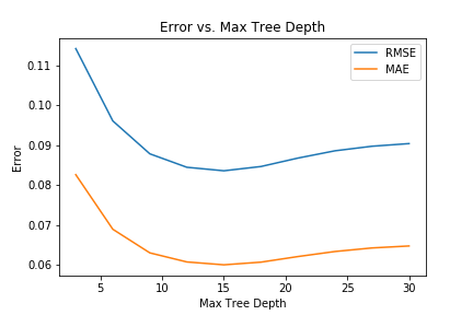
As stated earlier, the tree booster combines decision trees to form its ultimate model. As a result, one of its parameters is the maximum height of each tree. Since this booster yielded the lowest error, we decided to tune this hyperparameter to obtain the best model. Below is a graph of the MAE/RMSE errors as we increase the maximum tree depth input.
Analysis
We see that the best performance was observed on non pre-processed data, both in terms of faster training and lower error. This may be explained from the fact that XGBoost is known to work well with data that hasn’t gone through any modification.
Out of all 3 boosters tested, the one with best performance used simple decision trees as weak learners. The dart booster had very similar results, since it also uses trees, but may have added unnecessary complexity to the model, leading to slightly worse results. The linear model was much worse, and in general isn’t too common in gradient boosting. This may be because it is an oversimplified model, as its scope is only linear predictors.
For the maximum tree depth tuning, we see that the best value was at around 12. For lower values, the weak learners may be too simple to fit the data. It is also evident that after around a depth of 15, the errors start increasing, which is the result of overfitting due to the high complexity of the model
b. Neural Network
Architecture
We used a feedforward neural network with an input layer (fully connected to first hidden layer), 2 fully connected hidden layers and and an output layer to model the data and make a prediction for final PUBG placement. Below is an overview of the architecture used:
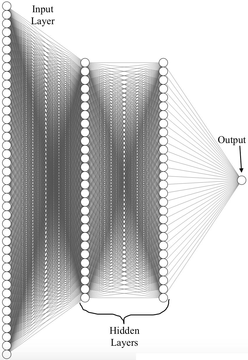
In the architecture, the size of the input layer is equal to the number of features in the input (size of the input vector) and the output layer has size 1 since we are outputting a single placement prediction. However, the size of the hidden layers is an important hyperparameter in neural networks that can be tuned. We experimented with different hidden layer sizes. In addition, we also ran extensive tests to determine optimal values for several other hyperparameters. Below we present an explanation of our approach for tuning different hyperparameters and the results used to determine optimal values.
Hyperparameter Tuning
Number of Hidden Units
The first hyperparameter we tuned is the number of hidden units (size of the hidden layers). We used all powers of 2 in the range [2, 256] as the hidden unit size and modeled the data using the resulting neural networ. We measured the Mean Absolute Error (MAE) for each configuration and determined that the optimal value is achieved when there are 32 hidden units in the hidden layers. Below is a plot of the results:
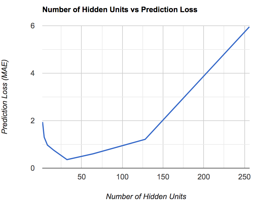
We note above that when the number of hidden units is too small, the model is not complex enough to capture the patterns in the data, thus leading to underfitting and high prediction error. Similarly, when the number of hidden units is too large, the model overfits the data which also produces high prediction error. Thus 32 seems to be the optimal value for the number of hidden units and the error is minimized.
Learning Rate
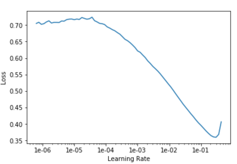
Another important hyperparameter in neural networks is the learning rate. The learning rate determines the step size along the gradient of the loss function at each iteration and as such impacts convergence. If the step size is too large, it is possible that we step over the minima and never reach it. If the step size is too small, then convergence might take extremely long and require multiple training iterations. When, the learning error was compared to the training loss, an optimal value of ~0.1 was observed as seen below:
Optimizer
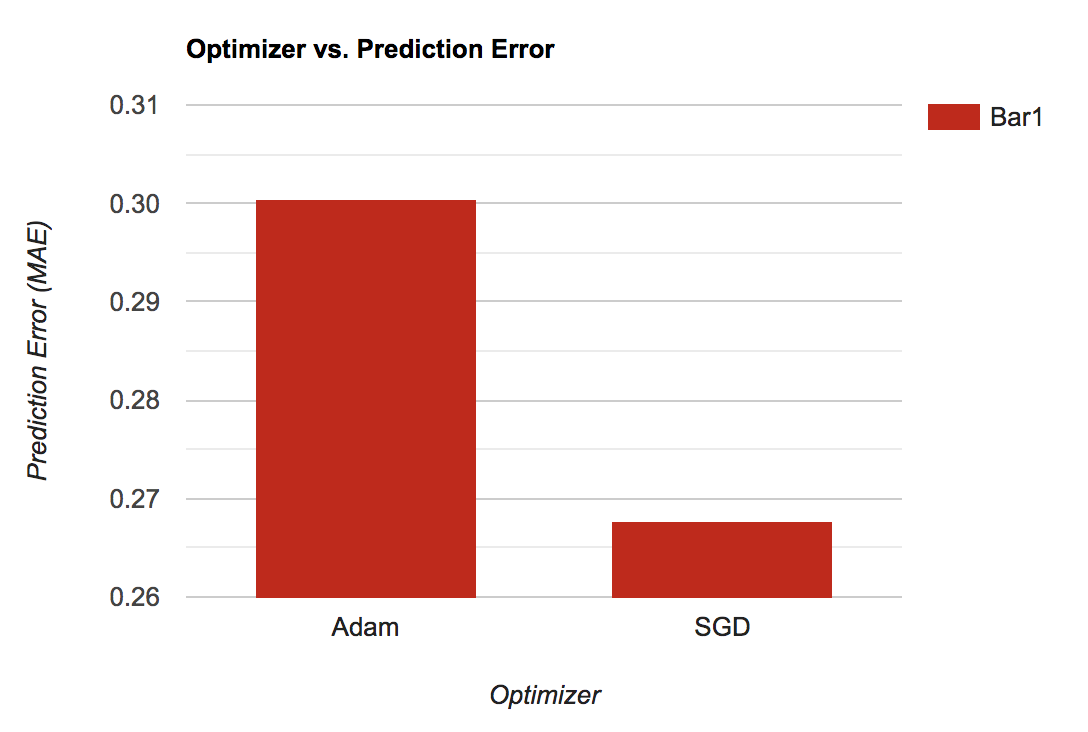
We also tested model performance (with 32 hidden units and learning rate of 0.1 - the optimal values determined from above) using two different optimizers: SGD and Adam (a popular deep learning optimizing algorithm). Optimizers control update steps along the gradient curve and as such also affect convergence rates and convergence to minima. SGD gave us better performance as seen below.
Results
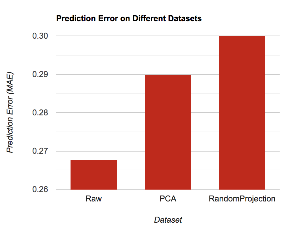
Using the optimal values for the hyperparameters determined above, we trained the model on the PUBG training dataset for 5 epochs. We ran the algorithm on the full dataset first and then on the dataset produced by the 2 dimension reduction methods mentioned above. The results we obtained are shown below:
Analysis
We see that we get the best performance on the raw dataset (no dimensionality reduction applied). This is reasonable because neural networks perform better when there is more data and more information (features) about the data. While dimensionality reduction methods get rid of closely related features, neural networks by their very nature of being universal function approximators are able to create higher level non-linear representations of even closely related fearures, thus leading to better performance. This is one of the reasons that many experts claim that feature engineering and feature selection are not of high importance when using neural networks and so this result is not surprising. Meanwhile, we notice that both the dimensionality reduction methods perform approximately the same with neural networks and that there is not a huge difference between the two different methods.
A note on the error function being used here: we are using MAE because the goal of this regression task is to output a percentile prediction for the finish position of a particular player. As such, we only care about how off we are from the true placement and not which direction we are off in. Hence, we made the choice of using MAE to measure performance. The Kaggle competition from where this dataset was obtained also uses MAE measure performance.
Conclusion
In summary, we used two unsupervised dimensionality reduction techniques: PCA and random projection to engineer our dataset and two supervised learning techniques: XGBoost and Deep Learning with Neural Networks to model the data and make predictions on final placement positions for PUBG players. We then compared performance of our two learning algorithms across three different datasets (original, PCA applied and random projection applied) to determine the best approach to this task. Our hope is to continue iterating on these models that we have built even beyond this class so that we can help competitive PUBG players identify the most important aspects of the game to focus on and improve to ensure high final placement. In doing so, we hope to be able to optimize our own playing strategies using the predictions of the model so that we can be competitive as a team.
References
- Howley, T., Madden, M. G., O’Connell, M.-L., & Ryder, A. G. (2006). The Effect of Principal Component Analysis on Machine Learning Accuracy with High Dimensional Spectral Data. Applications and Innovations in Intelligent Systems XIII, 209–222. doi: 10.1007/1-84628-224-1_16
- Tharwat, A., Gaber, T., Ibrahim, A., & Hassanien, A. E. (2017). Linear discriminant analysis: A detailed tutorial. AI Communications, 30(2), 169–190. doi: 10.3233/aic-170729
- Hornik, K., Stinchcombe, M. B., & White, H. (1989). Multilayer feedforward networks are universal approximators. Neural Networks, 2(5), 359-366. doi: 10.1016/0893-6080(89)90020-8
- Friedman, J. H. “Greedy Function Approximation: A Gradient Boosting Machine.” (Feb. 1999a)